All projectsDirectional speaker
Simulation
Solving KZK numerically
March the KZK equation with operator splitting, validate it, then drive it with a 60 kHz carrier modulated by 1 kHz and watch the air turn it into an audible, distorted tone.
Goals
- Explain operator splitting and why each sub-step can be solved exactly.
- Pass all four validation checks and explain what each one tests.
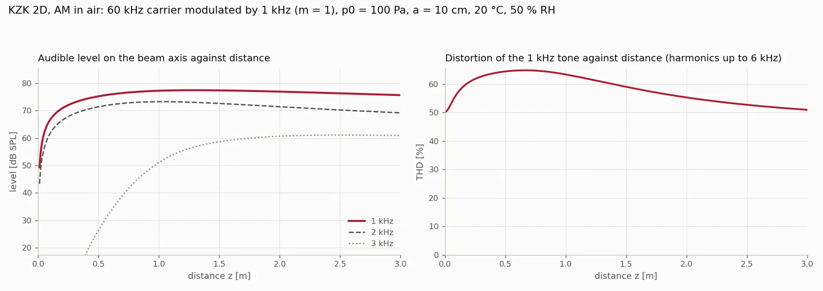
- Run the AM mode in air and read off the audible level and distortion against distance.
Why this matters
The simulation is how you predict what the speaker should sound like before you measure it, and later how you explain what you measured. A solver you have not validated is just a plot generator, so a good part of this step is proving the code right.
The physics
Split each step in into pieces that are each easy to solve exactly (Strang splitting: half nonlinear, full linear, half nonlinear):
- Diffraction and absorption. In the frequency domain each harmonic and transverse wavenumber evolves independently, so the linear step is just a phase and a decay, . In air comes from ISO 9613-1 for every harmonic separately, so the molecular-relaxation absorption is right at every frequency.
- Nonlinearity. has the implicit exact solution : every point of the waveform slides in in proportion to its pressure.
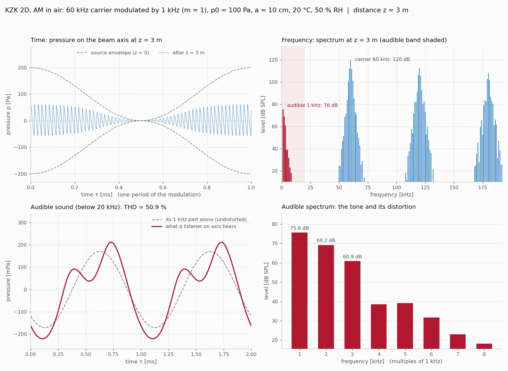
AM mode. The source is with kHz and kHz. The time window is one period of the audio, 1 ms, so “harmonic ” means kHz: the carrier is harmonic 60, and harmonics 1, 2, 3 are the audible tone and its distortion. The code low-passes the on-axis waveform below 20 kHz to get what a listener hears, and reports the total harmonic distortion .
Four analytic solutions check the code:
- A linear Gaussian beam, whose on-axis amplitude in 2D falls as .
- The Fubini solution for a lossless plane wave before shock formation, .
- The Fay solution for an old-age sawtooth, .
- An AM plane wave in air at short range, from second-order theory. For equal absorption of the carrier and sidebands it reduces to
In a plane wave the audio follows the first derivative of . Berktay’s second derivative only appears in the far field of a beam.
Hints
Hint 1Run the validation before anything else
python kzk_sim.py --validate should print ALL CHECKS PASSED. If you change the solver, run it again. The validation table belongs in your Methods section: it is the evidence that the later plots mean something.
Hint 2Watch it build up with distance
python kzk_gui.py --am opens the viewer in AM mode. Set the carrier, the tone and how far to go, then drag the distance slider to watch the audible tone appear, grow and distort, step by step. The other parameters (carrier amplitude, modulation index, source size, air temperature and humidity) are fixed in the viewer; change them with kzk_sim.py --am options if you need to.
Hint 3Turn the nonlinearity off
Run python kzk_sim.py --am 3 --linear. Where did the audible lines go? That one comparison shows the paper’s main idea: the air, not the speaker, makes the sound.
Hint 4Is that distortion real?
Plain AM with is expected to distort a lot. Second-order plane-wave theory gives , and Berktay’s far field gives . Where does your distance sit compared with the carrier’s Rayleigh distance , and does the THD land between the two?
Hint 5Try square-root AM
source_waveform() builds the envelope . Change it to and rerun. How much does the THD drop? Compare with what you measure from the department speaker.
Hint 62D is not the department’s speaker
The code models a strip source, so its beam spreads as while a real panel spreads as . Shapes and trends are meaningful; absolute levels need the axisymmetric version of the diffraction step.
What past teams did
2026–27 team
We wrote kzk_sim.py following Lee & Hamilton: FFTs in and for the linear step, a Newton-solved implicit shift for the nonlinear step, and an absorbing sponge at the transverse edges. Then we added the AM mode (--am), with ISO 9613-1 absorption for every harmonic and figures of the audible waveform, its spectrum and its THD. Two numerical lessons from that:
- The nonlinear step originally used linear interpolation, which smooths the waveform a little every step. That is harmless with ~1000 samples per period (the pure tone) but not with the ~64 samples per carrier cycle that the AM window allows, so AM mode uses cubic interpolation.
- The audible tone spreads much faster than the 60 kHz beam, so the transverse box has to be sized for the audio, not the carrier. Otherwise the audio reflects off the box edges and corrupts the result after a metre or two.
kzk_gui.py has both modes too: it imports the solver pieces from kzk_sim.py, so the two programs always use the same validated physics.